🍳 reference: <모두를 위한 딥러닝 2: pytorch> Lab2,3

import torch
import torch.nn as nn
import torch.nn.functional as F
import torch.optim as optim

1. Data Definition

공부 시간과 점수를 modeling한다고 가정하면,

training data는 (hours(x), points(y)), test data는 (hours)

x_train = torch.FloatTensor([[1], [2], [3]])
y_train = torch.FloatTensor([[2], [4], [6]])

2. Hypothesis

training data와 가장 잘 맞는 하나의 직선을 model 로 삼기

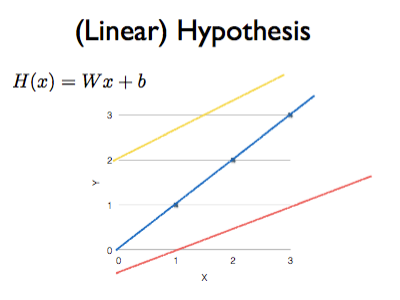
이때 W는 weight, b는 bias 이고 w와 b를 학습해야 한다.

W = torch.zeros(1, requires_grad=True)
b = torch.zeros(1, requires_grad=True)
hypothesis = x_train * W + b

처음에 w,b는 0으로 초기화해주고 requires_grad = True를 통해 앞으로 학습할 것이라 명시한다.

3. Compute Loss

cost

위와 같은 cost funtion은 아래와 같이 편하게 계산 가능하다

cost = torch.mean((hypothesis - y_train) ** 2)

4. Gradient descent

이제 SGD를 이용해 optimize를 하면 아래와 같다.

learning rate(lr)은 0.01이다

optimizer = optim.SGD([W, b], lr=0.01) # [W,b]가 학습할 tensor

optimizer.zero_grad() #gradient 초기화
cost.backward() # gradient 계산
optimizer.step() # 개선

Full code

# 데이터
x_train = torch.FloatTensor([[1], [2], [3]])
y_train = torch.FloatTensor([[1], [2], [3]])
# 모델 초기화
W = torch.zeros(1, requires_grad=True)
b = torch.zeros(1, requires_grad=True)
# optimizer 설정
optimizer = optim.SGD([W, b], lr=0.01)

nb_epochs = 1000
for epoch in range(nb_epochs + 1):

    # H(x) 계산
    hypothesis = x_train * W + b

    # cost 계산
    cost = torch.mean((hypothesis - y_train) ** 2)

    # cost로 H(x) 개선
    optimizer.zero_grad()
    cost.backward()
    optimizer.step()

    # 100번마다 로그 출력
    if epoch % 100 == 0:
        print('Epoch {:4d}/{} W: {:.3f}, b: {:.3f} Cost: {:.6f}'.format(
            epoch, nb_epochs, W.item(), b.item(), cost.item()
        ))

pytorch 의 model.mm으로 코드를 작성한다면, 아래와 같다

# 데이터
x_train = torch.FloatTensor([[1], [2], [3]])
y_train = torch.FloatTensor([[1], [2], [3]])
# 모델 초기화
model = LinearRegressionModel()
# optimizer 설정
optimizer = optim.SGD(model.parameters(), lr=0.01)

nb_epochs = 1000
for epoch in range(nb_epochs + 1):

    # H(x) 계산
    prediction = model(x_train)

    # cost 계산
    cost = F.mse_loss(prediction, y_train)

    # cost로 H(x) 개선
    optimizer.zero_grad()
    cost.backward()
    optimizer.step()

    # 100번마다 로그 출력
    if epoch % 100 == 0:
        params = list(model.parameters())
        W = params[0].item()
        b = params[1].item()
        print('Epoch {:4d}/{} W: {:.3f}, b: {:.3f} Cost: {:.6f}'.format(
            epoch, nb_epochs, W, b, cost.item()
        ))

Bias가 없는 model을 이용하여, GD를 더 자세히 이해해보자

x_train = torch.FloatTensor([[1], [2], [3]])
y_train = torch.FloatTensor([[1], [2], [3]])

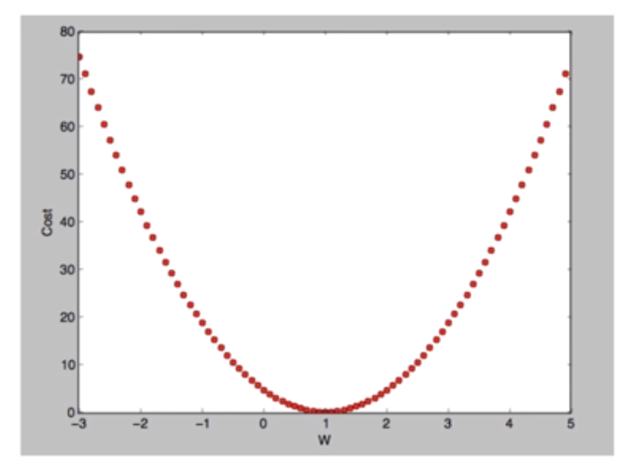
위 데이터에서, y = Wx의 W = 1이어야 정확한 예측이 가능하다

즉, w = 1에 가까울수록 좋은 모델이다

-> but, 이것을 어떻게 평가할까? cost(loss) function!

cost

이는 model의 예측값이 실제값과 얼마나 다른지를 나타냄 (정확할수록 0에 수렴)

아래와 같은 Mean Squared Error를 이용함

mse

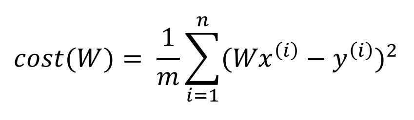
cost = torch.mean((hypothesis - y_train) ** 2)

이런 cost function을 최소화하기 위해, (정확한 학습을 위해)

기울기가 음수일때는 더 커져야 하고, 기울기가 양수일때에는 더 작아져야 한다

또한 기울기가 클수록 (가파를수록) w가 크게 바뀌고 작을수록 작게 바뀐다

이런 기울기 (= gradient)를 계산하기 위해선 아래와 같이 미분해야 한다.

이렇게 gradient를 이용해 cost function을 줄이는 것을 Gradient Descent라고 한다

# 데이터
x_train = torch.FloatTensor([[1], [2], [3]])
y_train = torch.FloatTensor([[1], [2], [3]])
# 모델 초기화
W = torch.zeros(1)
# learning rate 설정
lr = 0.1

nb_epochs = 10
for epoch in range(nb_epochs + 1):

    # H(x) 계산
    hypothesis = x_train * W

    # cost gradient 계산
    cost = torch.mean((hypothesis - y_train) ** 2)
    gradient = torch.sum((W * x_train - y_train) * x_train)

    print('Epoch {:4d}/{} W: {:.3f}, Cost: {:.6f}'.format(
        epoch, nb_epochs, W.item(), cost.item()
    ))

    # cost로 H(x) 개선
    ## 또는 W -= lr * gradient
    optimizer.zero_grad()
    cost.backward()
    optimizer.step()