[모두를 위한 딥러닝2 Pytorch] Perceptron, MLP
🍳 reference: <모두를 위한 딥러닝 2: pytorch> Lab8
Perceptron
인공신경망의 대표적인 예시인 Perceptron

위 그림에서 처럼 입력 x들과 가중치 w의 곱의 합에 bias를 더한 후 activation funtion을 거쳐 결과가 나온다.
초창기 perceptron은 linear classifier에 쓰였다.
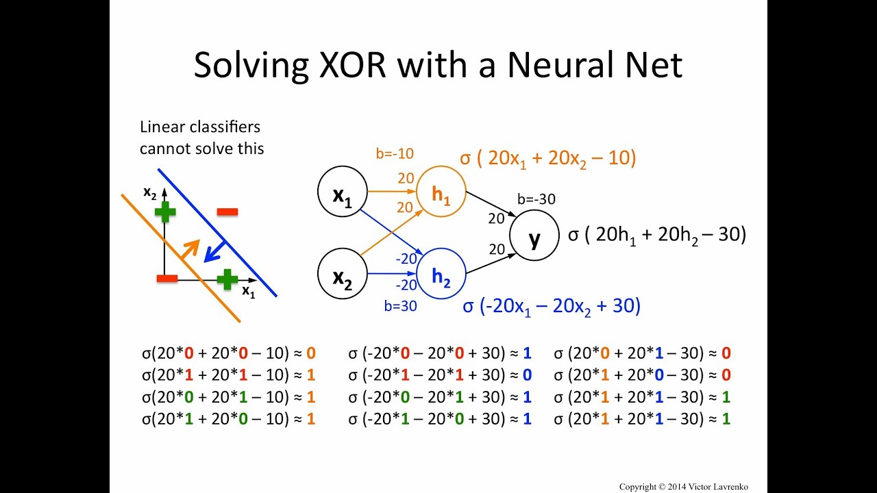
XOR
그러나 perceptron의 경우, XOR 문제를 해결하지 못했다.

그러나 XOR을 다른 방법으로 구현하게 되면서 딥러닝은 다시 bloom 했다!
일단 코드는 아래와 같다.
import torch

X = torch.FloatTensor([[0, 0], [0, 1], [1, 0], [1, 1]]).to(device)
Y = torch.FloatTensor([[0], [1], [1], [0]]).to(device)

# nn layers
linear = torch.nn.Linear(2, 1, bias=True)
sigmoid = torch.nn.Sigmoid()
# model
model = torch.nn.Sequential(linear, sigmoid).to(device)
# define cost/loss & optimizer
criterion = torch.nn.BCELoss().to(device) # BCELoss(): binary cross entropy loss 이용
optimizer = torch.optim.SGD(model.parameters(), lr=1)

for step in range(10001):
    optimizer.zero_grad()
    hypothesis = model(X)
    # cost/loss function
    cost = criterion(hypothesis, Y)
    cost.backward()
    optimizer.step()

    if step % 100 == 0:
        print(step, cost.item())
Multi Layer Perceptron (MLP)
단층이 아니라 여러 층으로 이루어진 perceptron을 의미한다.
MLP를 이용하여 아래와 같이 선을 하나 더 긋는 느낌으로 XOR 문제를 해결할 수 있었다.
물론 처음에는 MLP는 구현이 불가능했지만, backpropagation이 개발되면서 가능해졌다.
Backpropagation
xi들로 예측한 y는 실제 값과의 오차 loss 를 갖는다.
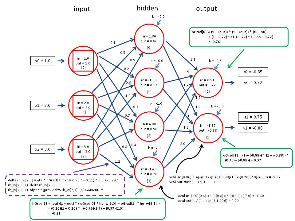
이를 weight에 대해 미분하여, 이를 이용해 뒤쪽 weight부터 loss를 최소화할 수 있도록 update 하는 것이다.
X = torch.FloatTensor([[0, 0], [0, 1], [1, 0], [1, 1]]).to(device)
Y = torch.FloatTensor([[0], [1], [1], [0]]).to(device)

# nn layers
w1 = torch.Tensor(2,2).to(device)
b1 = torch.Tensor(2).to(device)
w2 = torch.Tensor(2,1).to(device)
b2 = torch.Tensor(1).to(device)

def sigmoid(x):
  return 1.0/(1.0+torch.exp(-x))

def sigmoid_prime(x):
  return sigmoid(x)*(1-sigmoid(x))

for step in range(10001):
  # forward
  l1 = torch.add(torch.matmul(X, w1), b1)
  a1 = sigmoid(l1)
  l2 = torch.add(torch.matmul(a1, w2), b2)
  Y_pred = sigmoid(l2)

  cost = -torch.mean(Y*torch.log(Y_pred) + (1-Y)*torch.log(1-Y_pred))

  # Backpropagation (chain rule)
  ## Loss derivative
  d_Y_pred = (Y-Y_pred) / (Y_pred * (1.0 - Y_pred) + 1e-7)

  # Layer 2
  d_l2 = d_Y_pred * sigmoid_prime(l2)
  d_b2 = d_l2
  d_w2 = torch.matmul(torch.transpose(a1, 0, 1), d_b2)

  # Layer 1
  d_a1 = torch.matmul(d_B2, torch.transpose(w2, 0, 1))
  d_l1 = d_a1 * sigmoid_prime(l1)
  d_b1 = d_l1
  d_w1 = torch.matmul(torch.transpose(X, 0, 1), d_b1)

  # weight update
  w1 = w1-learning_rate * d_w1
  b1 = b1 - learning_rate * torch.mean(d_b1, 0)
  w2 = w2-learning_rate * d_w2
  b2 = b2 - learning_rate * torch.mean(d_b2, 0)

  if step%100 == 0: print(step, cost.item())
이러한 backpropagation을 이용한 XOR 코드는 아래와 같다.
X = torch.FloatTensor([[0, 0], [0, 1], [1, 0], [1, 1]]).to(device)
Y = torch.FloatTensor([[0], [1], [1], [0]]).to(device)

# nn layers
linear1 = torch.nn.Linear(2, 2, bias=True)
linear2 = torch.nn.Linear(2, 1, bias=True)
sigmoid = torch.nn.Sigmoid()

# model
model = torch.nn.Sequential(linear1, sigmoid, linear2, sigmoid).to(device)

# define cost/loss & optimizer
criterion = torch.nn.BCELoss().to(device)
optimizer = torch.optim.SGD(model.parameters(), lr=1)  # modified learning rate from 0.1 to 1

for step in range(10001):
    optimizer.zero_grad()
    hypothesis = model(X)

    # cost/loss function
    cost = criterion(hypothesis, Y)
    cost.backward()
    optimizer.step()

    if step % 100 == 0:
        print(step, cost.item())
또는 더 깊은 layer를 아래와 같이 설정할 수 있다. 이 경우 성능이 더 향상된다.
# nn layers
linear1 = torch.nn.Linear(2, 10, bias=True)
linear2 = torch.nn.Linear(10, 10, bias=True)
linear3 = torch.nn.Linear(10, 10, bias=True)
linear4 = torch.nn.Linear(10, 1, bias=True)
sigmoid = torch.nn.Sigmoid()

# model
model = torch.nn.Sequential(linear1, sigmoid, linear2, sigmoid, linear3, sigmoid, linear4, sigmoid).to(device)